10.1 Binary search trees
A binary search tree (BST) is a binary tree that satisfies the following invariant:
Invariant: Binary search trees
For every node with value v:
- all values in the left subtree are smaller than v, and
- v is smaller than all values in the right subtree.
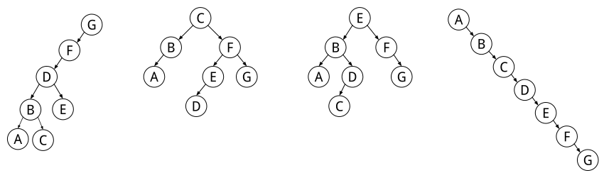
The only thing that differentiates a BST from a normal binary tree is this invariant. As explained in Section 3.2, an invariant is a condition that the BST always must satisfy. This means that the example tree from Section 9.1 is not a BST, because it violates the invariant, but Figure 10.1 shows four correct BSTs. Note that all these trees represent the same set of values, which means that if we use them to implement a set, then they should be indistinguishable for the program that makes use of them. However, there is one important difference between the four trees: the middle ones are much more balanced than the other two, and this has consequences for the efficiency of the basic operations.
10.1.1 Implementing BST sets and maps
In most programming languages it is not possible to specify invariants, but it is the responsibility of the programmer to make sure that the invariants are never violated.
Note that the BST invariant implies that all values in the tree are distinct from each other, which is exactly what we need to implement a set. Therefore, to implement a set we can reuse the binary tree implementation from Section 9.1:
datatype BST:
    root = null   // Pointer to the root node of the tree
    size = 0      // Size of the tree

datatype BSTNode:
    left     // Pointer to left child
    right    // Pointer to right child
    value    // Value for this node
Implementing multisets
A multiset, or a bag, is a collection of values that allows duplicates. This is easy to implement as a BST, we just have to relax the invariant a little. Instead of requiring that all children are unequal to the node value, we can say that the left children are smaller or equal to the parent, while the right children are still always larger. (It is just a convention that we let the left children be equal – we could also mirror it.)
Implementing maps
Now, how can we implement a map using a BST? The only difference to a normal BST is that the nodes have to both a key and a value:
datatype BSTMapNode:
    left      // Pointer to left child
    right     // Pointer to right child
    key       // Key for this node
    value     // Value for this node
The BST invariant should now only mention the keys in the subtrees, not the values. This is the only difference between a map and a set, implemented as BSTs. In the rest of this chapter we will mainly talk about how to implement sets, and we trust that you are experienced enough to be able to modify the data structures and algorithms to implement maps.
10.1.2 Searching in and adding to a BST
Because of the BST property, we do not have to search the whole tree if we want to find an element. Instead, we can start at the root node and compare its value with the value we are searching for. If the value is smaller than the root, we can continue searching in the left subtree. (And conversely, if the value is larger, we can search in the right subtree.) We continue searching until we have found the value in a node, or until we reach an empty child. If we reach an empty child (a null node), we know that the value is not in the tree.
Algorithm: Searching in a BST
To search a BST for a value x, we initialise a pointer to the root node, and repeat the following:
- If the pointer is an empty (null) node, return failure.
- Compare x with the value of the
pointed node:
- If they are equal, return success.
- Otherwise, move the pointer to the left or right child, depending on if x is smaller or larger than the node value.
Searching in a BST can also be done recursively, and here is an
interactive explanation of this.
Here is an exercise on searching in a BST.
How do we add a value to a BST? First of all we have to search for it. If the value is already in the tree we do nothing, and if it doesn’t exist we create a new node and attach it to the right place. But how do we know where to add the new node? After the search is finished, the pointer points to an empty node so this is not useful. Insetad, we have to remember the previous node we looked at – and then we can attach the new node as a child. If the new value is smaller, we add the node as a left child, and if it is larger we add it as a right child.
Algorithm: Adding to a BST
To add a value x to a BST, initialise a current pointer to the root node, and a previous pointer to null. Then repeat the following until current points to null:
- Compare x with the value of
current:
- If they are equal, return and do nothing at all.
- Otherwise, set previous to current, and reassign current to the left or right child, depending on if x is smaller or larger.
Now create a new node with value x and attach it as follows:
- Attach it to the root if previous is null, or
- to the left or right child of previous, depending on if x is smaller or larger than previous.
If you think that it is clumsy to keep two pointers in the algorithm above, the recursive variant becomes very simple and compact:
Algorithm: Adding to a BST, recursive version
To add a value x to a BST node:
- If the node is empty, return a node node with value x.
- Compare x with the node value:
- If they are equal, return the node as it is.
- Otherwise, reassign the left or right child (depending on if x is smaller or larger) with the result of adding x to it.
How can we translate this high-level algorithm into working code? The important part here is to realise that the recursive function should return the updated tree, and then it is just a matter of reassigning the child. So the pseudocode becomes something like this:
addHelper(node, x) -> BSTNode:
    if node is null:
        return new BSTNode(x)
    else if x == node.value:
        return node
    else if x < node.value:
        node.left = addHelper(node.left, x)
    else if x > node.value:
        node.right = addHelper(node.right, x)
    return node
The recursive function above is actually not the “real” function for adding a value, but instead an internal helper function. The toplevel function will have to call the helper with the root as the argument, and also update the root with the result.
add(bst, x):
    bst.root = addHelper(bst.root, x)
Here is an interactive explanation of recursive insertion, this time
in a BST map.
Here is an exercise on BST insertion.
10.1.3 Deleting from a BST
Removing a node from a BST is a bit trickier than adding, but it is not too hard if we consider the possible cases one by one. The first we have to do is to find the node with the element we want to remove, using the standard search algorithm. Now there are three possible cases:
- If it is a leaf node, we can just remove the parent’s pointer to the node.
- If it has one single child, we simply point the parent’s pointer to the child node directly.
- If it has two children, we call it an inner node. This is a trickier case that we have to discuss further.
To delete an inner node in a BST we don’t actually delete the node, because then we would have to restructure the tree quite a lot. Instead we replace its value with another value. The question is which value can we replace with?
We know that all values in the left subtree are smaller than the value we want to delete. Of these values there is one which is the largest value, and if we delete this one from the left subtree we can put it in the parent node instead. So we replace the inner node value we want to delete with the largest of the values in the left subtree. (Alternatively, we can replace it with the smallest value from the right subtree. This is an equally good strategy, so we can just pick one of them.)
Wait a little, did we really solve anything by doing this? We want to delete a value, and to be able to do that we have to delete a value in a subtree…
Yes, this works because we know that the largest value in a BST is never an inner node! (And the same holds for smallest value.) So, when we delete the largest (or smallest) value in the subtree we know that we will have one of the two easy cases. This means that we will not have to continue deleting values indefinitely.
The next question is, how do we find the largest value in a tree? This is easy, we just go as far to the right as possible – then we will end up in the largest element. (And similar for the smallest value – we go as far to the left as possible.)
Example: Deleting from a BST
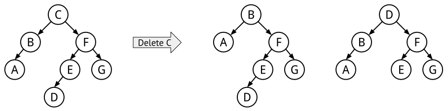
Suppose we want to delete the value C from the leftmost tree in Figure 10.2.
- First we find the C node, and the node with the largest value in the left subtree, which is the B node.
- We delete the B node, which means that we have to redirect the right child of its parent X to Y.
- Finally we can replace the value in the C node with B.
Alternatively, if we instead decide to replace with the smallest element in the right subtree:
- The node with the smallest value in the right subtree is the D node.
- We delete the D node, which means that we have delete the right child of its parent X.
- Finally we replace the value in the C node with D.
In the end we will get one of the two BSTs to the right in Figure 10.2. Notice that both of these trees are different representations of exactly the same set.
Now we are ready to formalise deletion into an algorithm.
Algorithm: Deleting a value in a BST
If we want to delete the value x in a BST, we first find the node that has that value. There are three possibilities for that node:
- If it is a leaf node, we can just delete it – meaning, deleting the corresponding child pointer of its parent.
- If the node has exactly one child, redirect its parent to the child.
- If it is an inner node, find the largest node y in the left subtree, and:
- Update the value of the x node to the value of the y node.
- Delete the y node from the left subtree.
How can we translate this algorithm into a working implementation? There are several possibilities, but we will show a recursive variant because the code becomes a bit less messy. One important thing to remember is that the recursive functions should return the updated tree, just as the recursive version of adding a value, from above. First we need a helper function for finding the largest value from a subtree:
findLargest(node):
    while node.right is not null:
        node = node.right
    return node.value
Finally, here is the main recursive function that deletes a value from a subtree:
removeHelper(node, value) -> BSTNode:
    if node is null:
        // We did not find the value, so do nothing.
    else if value < node.value:
        node.left = removeHelper(node.left, value)
    else if value > node.value:
        node.right = removeHelper(node.right, value)
    else if node has no children:
        node = null         // The node is a leaf, we can just delete it.
    else if node only has a left child:
        node = node.left    // Replace the node with its only child.
    else if node only has a right child:
        node = node.right   // Replace the node with its only child.
    else:   // Now we know that this is an inner node
        node.value = findLargest(node.left)      // Find the largest value in the left subnode,
        node.left = removeHelper(node.left, node.value)  // and delete this value.
    return node
And just as for recursive addition, we need to wrap this function in a toplevel call which starts with the tree root:
    remove(bst, x):
        bst.root = removeHelper(bst.root, x)
Here is an interactive explanation of BST deletion.
Here is an exercise on BST deletion.
10.1.4 Complexity analysis
The complexity of all basic operations all depend on how efficiently we can find the correct node, and this depends crucially on the structure of the tree.
When we search for an element we go down one level in the tree every time we compare with a node. So the worst case is when we search for a value that is in the lowest possible level, which is the same as the height of the tree. This means that the complexity of all basic operations is linear in the height, O(h). The height in turn depends on the tree structure:
- If the tree is balanced, meaning that all leaves are approximately on the same level, then the height is logarithmic in the number of nodes, and then searching is O(\log(n)). The middle trees in Figure 10.1 are examples of balanced trees.
- But if the tree us unbalanced, for example as the extremely left- and right-leaning trees in Figure 10.1, then the height is the same as the number of nodes, and search becomes linear O(n).
If we add values to a BST in sorted order (reversely sorted), then we get an extremely unbalanced tree. How long time will it take to build this tree? Assume that we add n values. Adding one value is in the worst case linear in n, and since we do this n times it will take quadratic time to build the final BST, O(n^2).
On the contrary, if we add the values in random order, then it is possible to prove that the final tree will have expected logarithmic height. Therefore, the operations will have expected worst-case complexity of O(\log(n)). And building the final BST with n values will be O(n\log(n)).
(This is similar to Quicksort with the simplest pivot, take-first, see Section 4.3. Sorting an already sorted array will take quadratic time, but if the list is randomly shuffled the complexity will be expected worst-case O(n\log(n)).)
In any case, almost noone uses plain BSTs because there is no guarantee of their worst-case complexity. But there are plenty of useful data structures that are based on BSTs and which have good worst-case guarantees. They accomplish this by automatically rebalancing themselves when necessary, and this is the topic of the next section.
10.1.5 Guided information flow
When writing a recursive function to solve a problem that requires traversing a binary tree, we want to make sure that we are visiting the required nodes (no more and no less).
In Section 9.1.3 we saw several tree traversals that visited every node of the tree, such as depth-first and breadth-first search. In this section we have also discussed searching, adding and removing in a BST, which each go down a single path of the tree. Guided traversal refers to problems that do not require visiting every node in the tree, though they typically require looking at more than one path through the tree. This means that the recursive function is making some decision at each node that sometimes lets it avoid visiting one or both of its children. The decision is typically based on the value of the current node. Many problems that require information flow on binary search trees are “guided” in this way.
Example: The number of values within a range
Assume that you want to know how many values there are in a BST that are within a given range. A bad solution to this problem would visit every node of the tree. However, we can take advantage of the BST invariant to avoid visiting unnecessary nodes. You know that the values greater than the root are always in the right subtree, and those values less than the root are in the left subtree. Therefore, we do not have to visit the left subtree at all if the node value is smaller than the minimum value in the range. And, conversely, we do not have to visit the right subtree if the node is larger than the range maximum.