12.7 Graph representation and implementation
There are two main ways of implementing graphs:
- Adjacency list
- A map from vertices to a list of its outgoing edges – this can be a BST, a hash table, or some other map data structure. If the vertices are exactly the numbers 0, 1, \ldots, n-1, the map can be a simple array (where the value of a vertex is the index in the array).
- Adjacency matrix
- A 2-dimensional matrix where the rows and columns denote vertices (assuming that the vertices are the numbers 0, 1, \ldots, n-1). A specific cell then denotes the edge from its column vertex to its row vertex – we can for example store the weight of the edge in the cell.
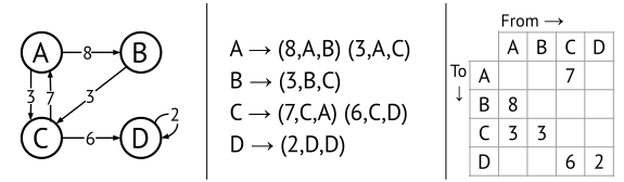
Figure 12.9 illustrates the
two representations. The adjecency list representation is simple and
very useful. The outgoingEdges function we have been using
in our graph algorithms corresponds to a lookup in the map, which can
make the operation very efficient. There are some things we can note
about the adjacency matrix representation:
- For an undirected graph, the matrix would be mirrored across the diagonal.
- For a sparse matrix, you end up with lots of empty cells.
- Finding the outgoing edges of a vertex is going to be O(V) even for very sparse graphs (you need to iterate through a column of the matrix and find all non-empty cells).
- If the graph was not weighted, its unclear what would be in the matrix, presumably just a boolean value.
Adjacency matrices are very handy for weighted graphs that are dense, providing a compact and fast implementation. The adjacency list is the most common for implementing generic sparse graphs.
There are plenty of optimisations possible for these representations. For instance, storing the source vertex in every edge is a bit redundant. For an unweighted graph, a compact adjacency map would just need to associate A with [B,C], saying that vertex A has edges to B and C. That is, unweighted graphs can be represented by a simple map from vertices to their adjacent vertices.