4.3 Quicksort
Mergesort uses a very simple approach for splitting the array, but spends almost all its time in the merging step. But there is also another problem with merging: it is difficult to efficiently implement in-place, so Mergesort has to use an additional array which will use some memory. So is there a different divide-and-conquer strategy that is easier to make in-place?
Quicksort uses another approach: it spends more of the time in splitting the array in parts, which then makes the merging step completely trivial. The overall algorithm is deceivingly similar to Mergesort:
Algorithm: Quicksort
To sort an array using Quicksort:
- Partition the array into two smaller parts,
- then recursively sort each part,
- finally concatenate the two parts into the final sorted array.
The main difference to Mergesort is in the splitting step, called partition. The idea is that we divide the array into two parts, where everything in the first part is smaller than everything in the second part. Then Quicksort calls itself with the two subarrays (just as Mergesort does), so that they are both sorted. Now we have to combine them, but this is much easier than in Mergesort, because we already know that everything in the first part is smaller than everything in the second part – so we can just put them after each other.
4.3.1 Partitioning
The biggest advantage of Quicksort over Mergesort is that partitioning can be done in-place, which merging cannot. And the main reason why we can partition in-place is because we can swap elements with each other.
To partition an array interval, we first select a pivot element from the interval. This is the value that decides which will elements go in the lower and upper parts. Now we create two pointers that start at the interval ends and then move towards each other. Whenever they encounter two elements that are in the wrong partition, they swap places. Or in other words: when the lower element is larger than the pivot, and the upper element is smaller than the pivot, the two elements swap places. When the pointers pass each other, the array has been partitioned.
There is one final detail we have to figure out before we have a complete algorithm: what should happen with the pivot? We know that in the end it must be in between the two partitions, but the problem is that we don’t know exactly how big the partitions will be – and therefore we cannot know in advance where to put the pivot. The standard solution is to first move the pivot out of the way – then partition the rest of the array, and afterwards put it back in. One good place to put it is at the beginning, so the first we do is to swap it there and then we partition the rest of the array. After the partitioning is finished and the pointers have passed each other, the upper pointer will point to the last element in the lower part. This is the final position of the pivot, so we can swap it into place.
Algorithm: Quicksort partition
To partition an array interval:
First, select some pivot element from the interval.
Swap the pivot with the first element in the interval, and initialise the lower and upper pointers to the second and last elements of the interval, respectively.
Repeat the following until the pointers have passed each other:
- Increase the lower pointer if its element is smaller than the pivot.
- Decrease the upper pointer if its element is larger than the pivot.
- Otherwise, swap the lower and upper elements, and move the pointers towards each other.
Swap the upper element with the pivot (which is now the first element in the interval).
Finally, Quicksort needs to know the final position of the pivot to be able to sort the two partitions recursively, so we have to return the upper pointer.
Here is a step-by-step example of partitioning.
First we select a pivot element:

Swap the pivot with the first element, and initialise the lower and upper pointers:
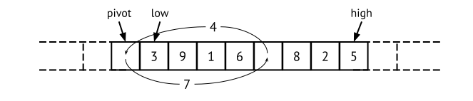
Partition the rest of the array. Move the pointers towards each other:

Whenever the lower element is larger than the pivot, and the upper element is smaller than the pivot, swap them:
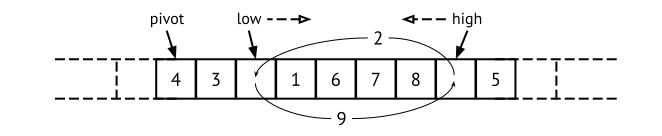
Finally, swap the pivot with the element at the upper pointer:
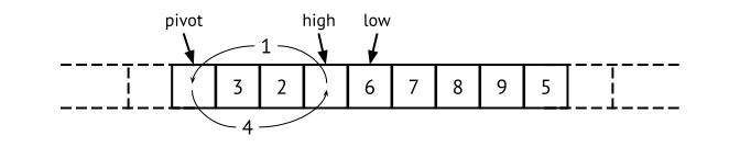
Return the new position of the pivot:
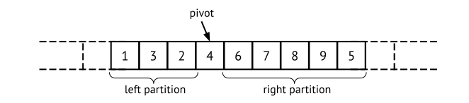
Note that the partitioning is done completely in-place. This is different from Mergesort where we need to allocate space for a temporary array.
After the partitioning is finished we know the following:
- The pivot is in its final position in the sorted array, so it will never have to be touched again.
- The left part is not sorted, but all the elements smaller than the pivot are present. This means that we can recursively sort the left part.
- The same for the right part.
Here is a visualisation of the partitioning algorithm. We assume that
we select the middle element as the pivot.
Quicksort partition proficiency exercise
Quicksort partition proficiency exercise
4.3.2 Categorising Quicksort
Compared to Mergesort, the partitioning process is completely in-place, but on the other hand we cannot be certain that the internal order between equal elements are preserved. This means that Quicksort is not a stable algorithm, and we have no guarantee for a good time complexity. Here is how we can categorise Quicksort according the three parameters from Section 2.1:
- In-place: yes, we do not have to create any intermediate arrays.
- Stable: no, equal elements might change order.
- Adaptive: yes, but it the complexity will never be better than linearithmic, O(n\log(n)).
Selection sort as a variant of Quicksort
What happens if we are extremely unlucky (or stupid) with the pivot selection?
Let us say that we always select the smallest possible pivot. This means that the lower partition will always be empty, and the upper partition will decrease by one in each step. The first time we will find the smallest element and put it first in the array. The second time we will find the second smallest element and put it after the first. Next time we will find the third smallest element and put it after the second, and so on.
This is exactly how Selection sort works! So conceptually, we can view Selection sort as a corner case of Quicksort, where we partition very unevenly.
4.3.3 Implementing Quicksort
Now we’re almost ready to implement Quicksort, but one small but important thing remains. We cannot know how big the left and right partitions will be, not until we have done the partitioning. So the partition function has to inform Quicksort how the partitions ended up – and we do this is to return the final position of the pivot. So here is the final algorithm sketch for sorting the interval \mathit{start}\ldots\mathit{end} of a given array:
- Select an initial index p_0 of the pivot, from the interval \mathit{start}\ldots\mathit{end}.
- Partition the interval using the pivot. Assume that the pivot has afterwards moved to position p.
- Sort the interval \mathit{start}\ldots p{-}1 and the interval p{+}1\ldots\mathit{end}.
Note that we do not include the pivot itself in the intervals of the recursive calls. This is because we know that after partitioning the pivot is in its final correct position, p. Now it should be straightforward to give the pseudocode for the main Quicksort function:
// Sort the array interval start...end
quickSort(arr, start, end):
    if start >= end:                       // Base case: Interval length is ≤ 1.
        return
    p0 = findPivot(arr, start, end)        // Pick an initial pivot index.
    p = partition(arr, start, end, p0)     // Partition the interval and update the pivot index.
    quickSort(arr, start, p-1)             // Quicksort the lower partition.
    quickSort(arr, p+1, end)               // Quicksort the upper partition.
The partitioning will return the final position of the pivot, which is the correct position of the pivot in the final, sorted array. By doing so, we guarantee that at least one value (the pivot) will not be included in the recursive calls. So even if a bad pivot is selected, yielding a completely empty partition to one side of the pivot, the larger partition will still contain one less element than the input array.
Implementing partitioning
The informal algorithm in Section 4.3.1 can be implemented as pseudocode like this:
partition(arr, start, end, p) -> Int:
    swap(arr, start, p)              // Put the pivot at the start of the interval.
    pivot = arr[start]               // Remember the pivot value, and
    low = start + 1; high = end      // initialise the lower and upper pointers.
    while low <= high:               // Continue until the pointers pass each other.
        if arr[low] < pivot:
            low += 1                 // Increase lower pointer if smaller than the pivot.
        else if arr[high] > pivot:
            high -= 1                // Decrease upper pointer if larger than the pivot.
        else:
            swap(arr, low, high)     // Otherwise, swap the elements, and
            low += 1                 // move both pointers towards each other.
            high -= 1
    swap(arr, start, high)           // Finally, swap the pivot into place, and
    return high                      // return the new position of the pivot.
You might wonder why we swap the pivot with the value at the upper pointer, why not swapping with the lower pointer? This is because we started by putting the pivot at the start of the interval. An equally good alternative partitioning algorithm would be to first swap the pivot with the end of the interval – but in that case we would have to do the final swap with the pivot with the lower pointer.
Here is a visualisation for the entire Quicksort algorithm.
This visualisation shows you how the logical decomposition caused by the partitioning process works. In the visualisation, the separate sub-partitions are separated out to match the recursion tree. In reality, there is only a single array involved (as you will see in the proficiency exercise that follows the visualisation).
Here is a complete proficiency exercise to see how well you
understand Quicksort.
Invariants for partitioning
In Section 3.2 we introduced invariants as a way of making algorithms precise and easier to reason about. This is very useful when implementing partitioning, because it can be difficult to understand the relation between the pointers start, low, high, and end.
Invariant: After each iteration of the
while-loop, the following invariants always hold:
- everything in the interval start+1…low-1 is smaller or equal to the pivot
- everything in the interval high+1…end is larger or equal to the pivot
4.3.4 Selecting a pivot
Perhaps the most important choice in implementing Quicksort is how to choose the pivot. Choosing a bad pivot can result in all elements of the array ending up in the same partition, in which case Quicksort ends up taking quadratic time.
The best is to select the median value (that is, not the average and not the middle value). This will make the two partitions the same size and we will get the best performance. In this case the complexity analysis is exactly the same as for Mergesort, because each recursive step divides the interval in two halves. Therefore Quicksort is linearithmic, O(n \log(n)), but only if we always select a good pivot.
However, it is difficult to find the median efficiently – we do not want to scan the whole array before we start partitioning, because this takes time. Instead we have to use some approximation.
First or last element
Choosing the first or the last element of the array interval is a very simple strategy, but it is also bad. If the input array is sorted, then the first element of the interval will also be the smallest (and the last will be the largest). Hence all elements of the array will end up in one of the partitions. Worse, exactly the same thing will happen in all the recursive calls to Quicksort. Hence the partitioning will be as bad as possible, and Quicksort will end up taking quadratic time.
The take-first or take-last strategy is also bad if the input is almost sorted, because the partitions will be very uneven in size and this is not good for Quicksort.
Middle element
A much better alternative is to pick the middle element of the interval. This makes partitioning behave very nicely sorted arrays, and on almost-sorted arrays. However, it is still very easy for a hacker to fool this strategy, so in practice, we have to use more sophisticated strategies.
Median-of-three
Even better is to look at a sample of the elements and pick the median of those. By far the most common is to take the median of the first, middle and last elements. This strategy is called median-of-three.
For example, given the array [3, 1, 4, 1, 5, 9, 2], we pick out the elements 3 (first position), 1 (middle position) and 2 (last position). The median of 3, 1 and 2 is 2, so we pick 2 as the pivot.
Median-of-three is not guaranteed to pick a good pivot: there are cases where it partitions the input array badly. However, these bad cases do not seem to occur in practice, so median-of-three is used by many real-world Quicksort implementations.
Non-well-behaved input
However, whatever strategy we have for choosing the pivot there is a risk that we are unlucky. In other words, there are always arrays that will make the strategy select a bad pivot. This is usually not a problem if the data is “well-behaved” – the pivot selected by the take-middle or median-of-three strategy will be close to optimal, and Quicksort will be as the name says, quick.
The problem arises as soon as you are not 100% certain where the data comes from. For example, if you implement a database that is connected to the internet, it can be exploited by a malicious hacker. If they know what strategy you use they can design input that will make your Quicksort algorithm quadratic instead of almost linear, and then bombard your database with such inputs which will make your server slow down to a halt.
Random pivot
So, how can we find a good pivot that is secure to hackers? One simple approach is to select a random element from the interval. This makes it extremely improbable that we will always get poor partitionings. In fact, it is possible to prove that the expected worst-case complexity of Quicksort with random pivot selection is linearithmic, O(n\log(n)).
Quicksort pivot proficiency exercise
Quicksort pivot proficiency exercise
In this exercise you should select which is the pivot element, if you always use the middle one.
4.3.5 Complexity analysis
To analyse Quicksort, we first analyse the functions for finding the pivot and partitioning an interval of length k. All the pivot selection strategies above take constant time for any k, so the total cost of partitioning is constrained by how far the lower and upper pointers can move towards each other.
- In each step of the
while-loop, either low or high (or both) moves one step. - Since the pointers always move towards each other, it will take at most k steps until they meet.
- So, the running time of the partition function is O(k).
Here is a visualisation illustrating the running time analysis of the
partition function.
Worst-case complexity
Quicksort’s worst case will occur when the pivot does a poor job of breaking the array, that is, when one partition becomes empty, and the other contains n-1 elements.
- The pivot partitions the array into two parts: one of size 0 and the other of size n-1. This requires n-1 units of work.
- In the second level, the pivot breaks it into two parts: one of size 0 and the other of size n-2. This requires n-2 units of work.
- In the third level, the pivot breaks it into two parts: one of size 0 and the other of size n-3. This requires n-3 units of work.
- And so on until the last level, where the pivot breaks a partition of size 2 into two parts: one of size 0 and the other of size 1. This requires a single unit of work.
Thus, the total amount of work is determined by the summation:
\sum_{i=1}^{n} i = \frac{1}{2} n (n-1) \; \in \; O(n^2)
This visualisation explains the worst-case running time of
Quicksort
So, the worst case running time of Quicksort is O(n^2). This is terrible, no better than Insertion or Selection sort. When will this worst case occur? Only when each pivot yields a bad partitioning of the array. If the pivot values are selected at random, then this is extremely unlikely to happen. If we instead always select the middle element in the interval, it is still unlikely to happen on well-behaved data. It does not take many good partitionings for Quicksort to work fairly well.
Best-case complexity
In Section 3.5 we argued why we usually are not interested in the best-case complexity, but Quicksort is an exception to this. It is interesting and useful to analyse the best-case complexity of Quicksort, because the best case is so much more common than the worst case (in normal circumstances). The very best case occurs if we always selects the best possible pivot, which is the one that always partitions the array into equal-sized parts.
- The pivot partitions the array into two halves of size n/2 each. This requires O(n) amount of work.
- For each of the two partitions, the pivot breaks it into halves of size n/4 each. This requires O(n) amount of work.
- For each of the four partitions, the pivot breaks it into halves of size n/8 each. This requires O(n) amount of work.
- And so on until the last level, where we reach n partitions each of size 1. This requires O(n) amount of work.
Note that this is exactly the same reasoning as for Mergesort. Thus, for each level, all partition steps for that level do a total of O(n) work. And if we always can find the perfect pivot, there will be only \log_2(n) levels. So the best-case running time of Quicksort is O(n \log(n)).
This visualisation explains the best-case running time of
Quicksort
Average-case complexity
Quicksort’s average-case behaviour falls somewhere between the extremes of worst and best case. Average-case analysis considers the cost for all possible arrangements of input, and calculates the average cost, weighted by how the data is distributed. As we already discussed in Section 3.5, the average case is extremely difficult to reason about, because real-world data does not usually have an even distribution.
For Quicksort it is possible to show that the number of “bad” cases are quickly outnumbered by the number of “good” cases, when the array size grows. This means that for well-behaved input, the average-case complexity of Quicksort is very likely to be closer to the best case than the worst case. In fact, if we select a random pivot in every step, then we can prove that the expected worst-case complexity is linearithimc, O(n\log(n)).
Inferring the complexity with a random pivot
Inferring the complexity with a random pivot
If we use a random pivot, then at every step, the pivot is equally likely to end in any position in the array. In other words, the pivot is equally likely to break an array into partitions of sizes 0 and n-1, or 1 and n-2, and so on. Now the average-case cost T(n) can be computed from the following equation:
\begin{align*} T(n) &= cn + \frac{1}{n}\sum_{k=0}^{n-1}[T(k) + T(n - 1 - k)] \\ T(0) = T(1) &= c \end{align*}
The equation above is a recurrence relation, and we will discuss those in more detail in Section 7.3. This visualisation will help you to understand how the recurrence relation was formed.
4.3.6 Variants and optimisations
In this section we discuss some variants of Quicksort, and things we can do to improve its efficiency.
Shuffle the array
As we explained above, if we use a random pivot we get a good asymptotic behaviour, because the expected worst-case complexity will be O(n\log(n)).
One alternative to using a random pivot is to shuffle the array before sorting, that is, rearranging it in random order. This only has to be done once before Quicksort begins, not in every recursive call. The advantage to doing this is that then we can safely use the simplest pivot selection strategy. And if we use the take-first pivot strategy we do not have to swap the pivot with the first element at the start of every partitioning. Depending on the computer and programming language, this can yield a slight improvement compared to using a random pivot.
Backing off to Insertion sort
A significant improvement can be gained by recognising that Quicksort is relatively slow when the array is small. This might not seem to be relevant if most of the time we sort large arrays, nor should it matter how long Quicksort takes in the rare instance when a small array is sorted because it will be fast anyway. But you should notice that Quicksort itself sorts many, many small arrays! This happens as a natural by-product of the divide and conquer approach.
A simple improvement is to replace Quicksort with a faster sort for smaller array intervals. This is a very common improvement, and usually one uses Insertion sort as the backoff algorithm. Now, at what size should we switch to Insertion sort? The answer can only be determined by empirical testing, but on modern machines the answer is probably somewhere between 10 and 100. Note that in Section 4.2.5 we discussed exactly the same improvement for Mergesort.
Running Insertion sort in a single final pass
There is a variant of the optimisation above: When Quicksort partitions are below a certain size, do nothing! The values within that partition will be out of order. However, we do know that all values in the array to the left of the partition are smaller than all values in the partition. All values in the array to the right of the partition are greater than all values in the partition. Thus, even if Quicksort only gets the values to “nearly” the right locations, the array will be close to sorted. This is an ideal situation in which to take advantage of the best-case performance of Insertion sort. The final step is a single call to Insertion sort to process the entire array, putting the records into final sorted order.
Alternative partitioning approaches
There are several possible ways we can translate the informal
partitioning algorithm into working code. For example, in our
implementation above we move the pointers at most one step in each
iteration of the while-loop. An alternative is to move the
pointers as far as possible during each iteration, and then the
pseudocode will become like this:
partition(arr, start, end, p) -> Int:
    swap(arr, start, p)          // Swap the pivot with the first element in the interval.
    pivot = arr[start]           // Remember the pivot value, and
    low = start + 1; high = end  // initialise the lower and upper pointers.
    repeat:
        while low <= high and arr[low] < pivot:
            low += 1             // Increase lower pointer as long as it's smaller than the pivot.
        while low <= high and arr[high] > pivot:
            high -= 1            // Increase upper pointer as long as it's larger than the pivot.
        if low > high:
            break                // Break out of loop when the pointers have passed each other.
        swap(arr, low, high)     // Otherwise, swap the elements, and
        low += 1                 // move both pointers towards each other.
        high -= 1
    swap(arr, start, high)       // Finally, swap the pivot into place, and
    return high                  // return the new position of the pivot.
This version is ever so slightly faster than the one in Section 4.3.3,
because in some cases it makes fewer comparisons. It is even possible to
improve this one a little bit more, because we do not need test
low<=high in the second inner while loop (try to reason
for yourself why that is the case).
The partitioning algorithm we described previously is called Hoare partitioning (named after the computer scientist C.A.R. Hoare). There is another common partitioning algorithm, where both pointers start at the left side and move to the right – but one of them moves faster than the other. This algorithm is called Lomuto partitioning (named after Nico Lomuto). In this algorithm we still have two pointers, but both start at the beginning of the array interval and move upwards. Below we call them \mathit{low} and \mathit{high}, where \mathit{low}\leq\mathit{high}. The invariant is that the elements from \mathit{start} to \mathit{low}-1 are always less than the pivot, and the elements from \mathit{low} to \mathit{high} are greater than or equal to the pivot. In Lomuto’s partitioning scheme we start by putting the pivot at the end of the interval, not the beginning.
partition(arr, start, end, p) -> Int:
    swap(arr, p, end)             // Swap the pivot with the last element in the interval.
    pivot = arr[start]            // Remember the pivot value, and
    low = start                   // initialise the lower pointer.
    for high in start .. end-1:   // Iterate the upper pointer over the entire interval.
        if arr[high] <= pivot:
            swap(arr, low, high)  // Swap lower and upper elements if upper is smaller than pivot,
            low += 1              // and increase the lower pointer.
    swap(arr, end, low)           // Finally, swap the pivot into place, and
    return low                    // return the new position of the pivot.
As you can see, Lomuto’s partitioning scheme gives very simple and clean implementation, but it is usually somewhat less efficient than Hoare’s, because it makes more swaps. It also does not work very well if the array contains many equal elements.
Three-way quicksort
If the array contains many equal elements, there is a small optimisation we can do to the partitioning scheme. Our current formulation divides the array into one lower part, then the pivot, and finally the upper part. If the array happens to contain many duplicates of the pivot, it would be useful to put all of them next to each other. This means that the algorithm divides the array into three parts: the lower part, the equal part, and the upper part. Our partitioning algorithm then has to return two indices, giving the end of the lower part and the beginning of the upper. Assuming that we have such an algorithm, the final Quicksort algorithm can be described like this:
- Select an initial pivot from the interval \mathit{start}\ldots\mathit{end}.
- Partition the interval using the pivot. Assume that the partitioning returns the positions p (the end of the lower part) and q (the start of the upper part).
- Sort the interval \mathit{start}\ldots p and the interval q\ldots\mathit{end}.
Three-way partitioning is also called the Dutch national flag problem, and the most common algorithm for solving it is a modification the Lomuto partitioning scheme from above.