9.6.1 Prim’s Algorithm

The first of our two algorithms for finding MCSTs is commonly referred to as Prim’s algorithm. Prim’s algorithm is very simple. Start with any Vertex $N$ in the graph, setting the MCST to be $N$ initially. Pick the least-cost edge connected to $N$. This edge connects $N$ to another vertex; call this $M$. Add Vertex $M$ and Edge $(N, M)$ to the MCST. Next, pick the least-cost edge coming from either $N$ or $M$ to any other vertex in the graph. Add this edge and the new vertex it reaches to the MCST. This process continues, at each step expanding the MCST by selecting the least-cost edge from a vertex currently in the MCST to a vertex not currently in the MCST.

Prim’s algorithm is quite similar to Dijkstra’s algorithm for finding the single-source shortest paths. The primary difference is that we are seeking not the next closest vertex to the start vertex, but rather the next closest vertex to any vertex currently in the MCST. Thus the following lines in Djikstra’s algorithm:

dist = D.get(v) + e.weight
if dist < D.get(w):
    D.put(w, dist)

are replaced with the following lines in Prim’s algorithm:

if e.weight < D.get(w):
    D.put(w, e.weight)

The following code shows an implementation for Prim’s algorithm that searches the distance matrix for the next closest vertex.

// Compute shortest distances to the MCST, store them in D.
// parent.get(v) will hold the index for the vertex that is v's parent in the MCST
function Prim(G, s):
    visited = new Set()
    parent = new Map()
    D = new Map()
    for each v in G.vertices():
        D.put(v, ∞)
    D.put(s, 0)

    repeat G.vertxCount() times:  // Process the vertices
        v = minVertex(G, D, visited)  // Find next-closest vertex
        visited.add(v)
        if D.get(v) == ∞:
            return parent
        for each e in G.outgoingEdges(v):
            w = e.end
            if e.weight < D.get(w):
                D.put(w, e.weight)
                parent.put(w, v)
    return parent

For each vertex e, when e is processed by Prim’s algorithm, an edge going to e is added to the MCST that we are building. Array V[e] stores the previously visited vertex that is closest to Vertex e. This information lets us know which edge goes into the MCST when Vertex e is processed.

9.6.2 Prim’s Algorithm, Priority Queue Implementation

Alternatively, we can implement Prim’s algorithm using a priority queue to find the next closest vertex, as shown next. As with the priority queue version of Dijkstra’s algorithm, the heap stores DijkElem objects.

// Prim's MCST algorithm: priority queue version
function PrimPQ(G, s):
    visited = new Set()
    parent = new Map()
    D = new Map()
    for (v : G.vertices())
        D.put(v, ∞)
    D.put(s, 0)

    agenda = new PriorityQueue()
    agenda.add(new KVPair(0, s))

    while not agenda.isEmpty():
        v = agenda.removeMin().value
        if v not in visited:
            visited.add(v)
            if D.get(v) == ∞:
                return parent
            for each e in G.outgoingEdges():
                w = e.end
                if e.weight < D.get(w):
                    D.put(w, e.weight)
                    parent.put(w, v)
                    agenda.add(new KVPair(e.weight, w))
    return parent

Prim’s algorithm is an example of a greedy algorithm. At each step in the for loop, we select the least-cost edge that connects some marked vertex to some unmarked vertex. The algorithm does not otherwise check that the MCST really should include this least-cost edge. This leads to an important question: Does Prim’s algorithm work correctly? Clearly it generates a spanning tree (because each pass through the for loop adds one edge and one unmarked vertex to the spanning tree until all vertices have been added), but does this tree have minimum cost?

Theorem: Prim’s algorithm produces a minimum-cost spanning tree.

Proof: We will use a proof by contradiction. Let $\mathbf{G} = (\mathbf{V}, \mathbf{E})$ be a graph for which Prim’s algorithm does not generate an MCST. Define an ordering on the vertices according to the order in which they were added by Prim’s algorithm to the MCST: $v_0, v_1, ..., v_{n-1}$. Let edge $e_i$ connect $(v_x, v_i)$ for some $x < i$ and $i \leq 1$. Let $e_j$ be the lowest numbered (first) edge added by Prim’s algorithm such that the set of edges selected so far cannot be extended to form an MCST for $\mathbf{G}$. In other words, $e_j$ is the first edge where Prim’s algorithm “went wrong.” Let $\mathbf{T}$ be the “true” MCST. Call $v_p (p<j)$ the vertex connected by edge $e_j$, that is, $e_j = (v_p, v_j)$.

Because $\mathbf{T}$ is a tree, there exists some path in $\mathbf{T}$ connecting $v_p$ and $v_j$. There must be some edge $e'$ in this path connecting vertices $v_u$ and $v_w$, with $u < j$ and $w \geq j$. Because $e_j$ is not part of $\mathbf{T}$, adding edge $e_j$ to $\mathbf{T}$ forms a cycle. Edge $e'$ must be of lower cost than edge $e_j$, because Prim’s algorithm did not generate an MCST. This situation is illustrated in Figure #PrimProof. However, Prim’s algorithm would have selected the least-cost edge available. It would have selected $e'$, not $e_j$. Thus, it is a contradiction that Prim’s algorithm would have selected the wrong edge, and thus, Prim’s algorithm must be correct.

Figure: Proof of Prim’s algorithm

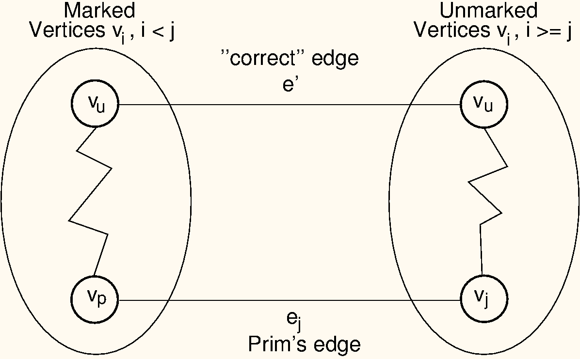
Prim’s MCST algorithm proof. The left oval contains that portion of the graph where Prim’s MCST and the “true” MCST $\mathbf{T}$ agree. The right oval contains the rest of the graph. The two portions of the graph are connected by (at least) edges $e_j$ (selected by Prim’s algorithm to be in the MCST) and $e'$ (the “correct” edge to be placed in the MCST). Note that the path from $v_w$ to $v_j$ cannot include any marked vertex $v_i, i \leq j$, because to do so would form a cycle.

9.6.3 Kruskal’s Algorithm

Our next MCST algorithm is commonly referred to as Kruskal’s algorithm. Kruskal’s algorithm is also a simple, greedy algorithm. First partition the set of vertices into $|\mathbf{V}|$ disjoint sets, each consisting of one vertex. Then process the edges in order of weight. An edge is added to the MCST, and two disjoint sets combined, if the edge connects two vertices in different disjoint sets. This process is repeated until only one disjoint set remains.

The edges can be processed in order of weight by putting them in an array and then sorting the array. Another possibility is to use a minimum priority queue, similar to what we did in Prim’s algorithm.

The only tricky part to this algorithm is determining if two vertices belong to the same equivalence class. Fortunately, the ideal algorithm is available for the purpose – the UNION/FIND algorithm. Here is an implementation for Kruskal’s algorithm. Note that since the MCST will never have more than $|\mathbf{V}|-1$ edges, we can return as soon as the MCST contains enough edges.

// Kruskal's MCST algorithm
function Kruskal(G):
    A = new ParentPointerTree()
    for each v in G.vertices():
        A.MAKE_SET(v)  // Create one singleton set for each vertex

    edges = new PriorityQueue()
    for each v in G.vertices():
        for each e in G.outgoingEdges(v):
            edges.add(new KVPair(e.weight, e))

    numEdgesInMCST = 0
    while not edges.isEmpty():
        e = edges.removeMin()
        if A.FIND(e.start) != A.FIND(e.end):  // If the vertices are not connected...
            AddEdgetoMCST(edge)               // ...add this edge to the MCST
            numEdgesInMCST = numEdgesInMCST + 1
            if numEdgesInMCST >= G.vertexCount()-1:
                return A                      // Stop when the MCST has |V|-1 edges
            A.UNION(e.start, e.end)           // Connect the two vertices

Kruskal’s algorithm is dominated by the time required to process the edges. The FIND and UNION functions are nearly constant in time if path compression and weighted union is used. Thus, the total cost of the algorithm is $\Theta(|\mathbf{E}| \log |\mathbf{E}|)$ in the worst case, when nearly all edges must be processed before all the edges of the spanning tree are found and the algorithm can stop. More often the edges of the spanning tree are the shorter ones, and only about $|\mathbf{V}|$ edges must be processed. If so, the cost is often close to $\Theta(|\mathbf{V}| \log |\mathbf{E}|)$ in the average case (provided we use a priority queue instead of sorting all edges in advance).