13.10.1 All-pairs shortest paths: Floyd’s algorithm

We next consider the problem of finding the shortest distance between all pairs of vertices in the graph, called the all-pairs shortest paths problem. To be precise, for every $v, w \in \mathbf{V}$, calculate $d(v, w)$.

One solution is to run Dijkstra’s algorithm $|\mathbf{V}|$ times, each time computing the shortest path from a different start vertex. If $\mathbf{G}$ is sparse (that is, $|\mathbf{E}| \in O(|\mathbf{V}|)$) then this is a good solution, because the total cost will be $O(|\mathbf{V}|^2 + |\mathbf{V}||\mathbf{E}| \log |\mathbf{V}|) = O(|\mathbf{V}|^2 \log |\mathbf{V}|)$ for the version of Dijkstra’s algorithm based on priority queues. For a dense graph, the priority queue version of Dijkstra’s algorithm yields a cost of $O(|\mathbf{V}|^3 \log |\mathbf{V}|)$, but the version using minVertex yields a cost of $O(|\mathbf{V}|^3)$.

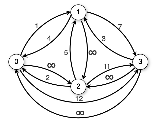
Another solution that limits processing time to $O(|\mathbf{V}|^3)$ regardless of the number of edges is known as Floyd’s algorithm. It is an example of dynamic programming. The chief problem with solving this problem is organising the search process so that we do not repeatedly solve the same subproblems. We will do this organisation through the use of the $k$-path. Define a k-path from vertex $v$ to vertex $w$ to be any path whose intermediate vertices (aside from $v$ and $w$) all have indices less than $k$. A 0-path is defined to be a direct edge from $v$ to $w$. Figure 13.13 illustrates the concept of $k$-paths.

Define $\mathrm{D}_k(v, w)$ to be the length of the shortest $k$-path from vertex $v$ to vertex $w$. Assume that we already know the shortest $k$-path from $v$ to $w$. The shortest $(k+1)$-path either goes through vertex $k$ or it does not. If it does go through $k$, then the best path is the best $k$-path from $v$ to $k$ followed by the best $k$-path from $k$ to $w$. Otherwise, we should keep the best $k$-path seen before. Floyd’s algorithm simply checks all of the possibilities in a triple loop. Here is the implementation for Floyd’s algorithm. At the end of the algorithm, array D stores the all-pairs shortest distances.

function floyd(graph):
    distances = new Map() of vertex pairs to distances
    for each v in graph.vertices():
        for each w in graph.vertices():
            distances.put((v, w), ∞)
        distances.put((v, v), 0)
        for each e in G.outgoingEdges(v):
            distances.put((v, e.end), e.weight)

    // Compute all k-paths
    for each k in graph.vertices():
        for each v in graph.vertices():
            for each w in graph.vertices():
                dist = distances.get(v, k) + distances.get(k, w)
                if dist < distances.get(v, w):
                    distances.put((v, w), dist)
    return distances

Clearly this algorithm requires $O(|\mathbf{V}|^3)$ running time, and it is the best choice for dense graphs because it is (relatively) fast and easy to implement.

13.10.2 Acyclic graphs: Topological sort

Assume that we need to schedule a series of tasks, such as classes or construction jobs, where we cannot start one task until after its prerequisites are completed. We wish to organise the tasks into a linear order that allows us to complete them one at a time without violating any prerequisites. We can model the problem using a DAG. The graph is directed because one task is a prerequisite of another – the vertices have a directed relationship. It is acyclic because a cycle would indicate a conflicting series of prerequisites that could not be completed without violating at least one prerequisite. The process of laying out the vertices of a DAG in a linear order to meet the prerequisite rules is called a topological sort.

Figure 13.14 illustrates the problem. An acceptable topological sort for this example is J1, J2, J3, J4, J5, J6, J7. However, other orders are also acceptable, such as J1, J3, J2, J6, J4, J5, J7.

function topsortDFS(graph):
    visited = new Set()
    sortedVertices = new Stack()
    for each v in graph.vertices():
        if v not in visited:
            topsortHelperDFS(graph, v, sortedVertices, visited)
    return sortedVertices

function topsortHelperDFS(graph, v, sortedVertices, visited):
    if v not in visited:
        visited.add(v)
        for each e in graph.outgoingEdges(v):
            topsortHelperDFS(graph, e.end, sortedVertices, visited)
        sortedVertices.push(v)  // postVisit

function topsortBFS(graph):
    // Initialise the prerequisite counts
    counts = new Map() of vertices to prerequisite count
    for each v in graph.vertices():
        counts.put(v, 0)
    for each v in graph.vertices():
        for each edge in graph.outgoingEdges(v):
            // Increase v's prerequisite count
            newCount = counts.get(edge.end) + 1
            counts.put(edge.end, newCount)

    // Initialise the queue
    queue = new Queue()
    for each v in graph.vertices():
        // Only add vertices that have no prerequisites
        if counts.get(v) == 0:
            queue.enqueue(v)

    // Process the vertices
    sortedVertices = new Queue()
    while not queue.isEmpty():
        v = queue.dequeue()
        sortedVertices.enqueue(v)  // preVisit
        for each e in graph.outgoingEdges(v):
            // Decrease v's prerequisite count
            newCount = counts.get(edge.end) - 1
            counts.put(edge.end, newCount)
            if newCount == 0:
                queue.enqueue(e.end)
    return sortedVertices