13.6.1 Priority queue implementation of Prim’s algorithm

An alternative approach is to store unprocessed vertices in a minimum priority queue, such as a binary heap, ordered by their distance from the processed vertices. The next-closest vertex can be found in the heap in $O(\log |\mathbf{V}|)$ time. Every time we modify $\mathbf{D}(X)$, we could reorder $X$ in the heap by deleting and reinserting it. This is an example of a priority queue with priority update. However, to implement true priority updating, we would need to store with each vertex its position within the heap so that we can remove its old distances whenever it is updated by processing new edges.

A simpler approach is to add the new (always smaller) distance value for a given vertex as a new record in the heap. The smallest value for a given vertex currently in the heap will be found first, and greater distance values found later will be ignored because the vertex will already be marked as visited. The only disadvantage to repeatedly inserting distance values in this way is that it will raise the number of elements in the heap from $O(|\mathbf{V}|)$ to $O(|\mathbf{E}|)$ in the worst case. But in practice this only adds a slight increase to the depth of the heap. The time complexity is $O((|\mathbf{V}| + |\mathbf{E}|) \log |\mathbf{E}|)$, because for each edge that we process we must reorder the heap.

Here is the implementation for Dijkstra’s algorithm using a priority queue.

function primPQ(graph, start):
    visited = new Set() of vertices
    parent = new Map() of vertices to vertices
    distances = new Map() of vertices to their distance from the MST
    agenda = new PriorityQueue() of vertices ordered by their distance from the MST
    // The distance from start to start is 0:
    distances.put(start, 0)
    agenda.add(start) with priority 0

    while not agenda.isEmpty():
        v = agenda.removeMin()
        if v not in visited:
            visited.add(v)
            for each e in graph.outgoingEdges():
                if e.end not in distances or dist < distances.get(e.end):
                    // If the edge makes the endpoint closer to the MST,
                    // update the endpoint with the new distance, add it to the MST and the agenda
                    distances.put(e.end, e.weight)
                    parent.put(e.end, v)
                    agenda.add(e.end) with priority e.weight
    return parent

13.6.2 Correctness of Prim’s algorithm

Prim’s algorithm is an example of a greedy algorithm. At each step in the for loop, we select the least-cost edge that connects some marked vertex to some unmarked vertex. The algorithm does not otherwise check that the MST really should include this least-cost edge. This leads to an important question: Does Prim’s algorithm work correctly? Clearly it generates a spanning tree (because each pass through the for loop adds one edge and one unmarked vertex to the spanning tree until all vertices have been added), but does this tree have minimum cost?

Theorem: Prim’s algorithm produces a minimum-cost spanning tree.

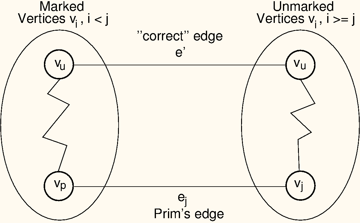
Proof: We will use a proof by contradiction. Let $\mathbf{G} = (\mathbf{V}, \mathbf{E})$ be a graph for which Prim’s algorithm does not generate an MST. Define an ordering on the vertices according to the order in which they were added by Prim’s algorithm to the MST: $v_0, v_1, ..., v_{n-1}$. Let edge $e_i$ connect $(v_x, v_i)$ for some $x < i$ and $i \leq 1$. Let $e_j$ be the lowest numbered (first) edge added by Prim’s algorithm such that the set of edges selected so far cannot be extended to form an MST for $\mathbf{G}$. In other words, $e_j$ is the first edge where Prim’s algorithm “went wrong.” Let $\mathbf{T}$ be the “true” MST. Call $v_p (p<j)$ the vertex connected by edge $e_j$, that is, $e_j = (v_p, v_j)$. Because $\mathbf{T}$ is a tree, there exists some path in $\mathbf{T}$ connecting $v_p$ and $v_j$. There must be some edge $e'$ in this path connecting vertices $v_u$ and $v_w$, with $u < j$ and $w \geq j$. Because $e_j$ is not part of $\mathbf{T}$, adding edge $e_j$ to $\mathbf{T}$ forms a cycle. Edge $e'$ must be of lower cost than edge $e_j$, because Prim’s algorithm did not generate an MST. This situation is illustrated in Figure 13.11. However, Prim’s algorithm would have selected the least-cost edge available. It would have selected $e'$, not $e_j$. Thus, it is a contradiction that Prim’s algorithm would have selected the wrong edge, and thus, Prim’s algorithm must be correct.

Here is an exercise for Prim’s algorithm.